Introduction to Exponential Smoothing

This article is an extract from the recent session ‘Intro to Time Series Forecasting’, presented at the Berlin Time Series Meetup:
https://www.meetup.com/Berlin-Time-Series-Analysis-Meetup/events/279676400/

Despite being discovered over 50 years ago, Exponential Smoothing (ETS) is still one of the workhorses of modern forecasting applications. In practice, ETS often proves to be very difficult to beat, regardless of its simplicity. This is particularly true for univariate (single variable) time series, where the practitioner knows little about the data generating process. In these cases, ETS proves to be a robust benchmarking method.

As evidence, consider the M4 Forecasting competition, run in 2018. The M-Series Forecasting competitions ask Data Scientists and Statisticians to submit their best models, in a competition to find the best forecasts across numerous time series. May the best model win.

In the 2018 contest, a benchmark model was submitted by the organisers consisting of an arithmetic mean of 3 ETS models. In fact, only 17 entrants were able to beat the ETS combination benchmark, despite having the choice of any model, of any complexity. While we won’t claim that ETS is the best or most powerful choice for forecasting, its simplicity and robustness makes it the go-to method for baseline forecasts. If your stacked combination of a Light-GBM and an LSTM can’t beat good old ETS, its back to the drawing board. In addition, ETS also requires few parameters to train and may still be the best choice for problems with very little data.

With that said, lets get into the meat and potatoes. In this article we will introduce 4 key variants of ETS. They are:

1. Simple Exponential Smoothing
2. Double Exponential Smoothing
3. Triple Exponential Smoothing
4. A small model adaption to handle exponential growth

In general, ETS has many variants and parameters and it would be impossible to cover them all in one article, however these 4 make a great starting point for a lot of practical applications.

Simple Exponential Smoothing

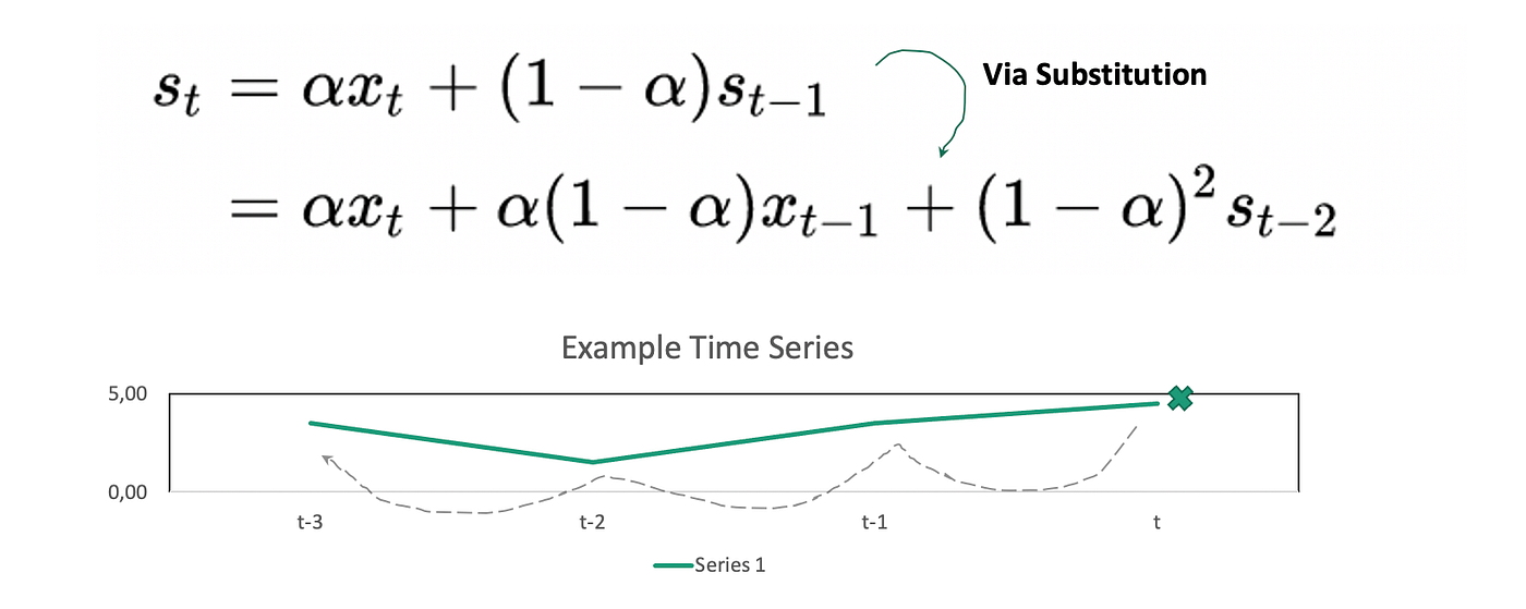
The formula for simple exponential smoothing is given below. It consists of a single parameter alpha, which determines how much of the time series history is used to forecast the next value. As you can see, the formula is also recursive. S_t-1 depends on S_t-2 and so on. This recursion is illustrated in the diagram. In the end, it is basically a weighted average of past values where the weights decrease exponentially over time.

Simple Exponential Smoothing

Lets now try out an example. To begin with we’ve prepared a simple time series (t1), which is shown in the image below. The time series is relatively flat, with fluctuations between -1 and 2.

Time Series #1

If we choose a low value of alpha and fit an ETS model, we get a smoother fit (because it incorporates more information from past values). If we select a larger alpha, we get a fit closer to the most recent value. This is illustrated below.

ETS Fit with Alpha = 0.2

ETS Fit with Alpha = 0.8

Using the first model (alpha = 0.2), we get the following forecasts:

Forecast of Time Series #1 using Simple Exponential Smoothing

This forecasts look reasonable. If you wanted to fine tune the model, you’d try to find the best possible alpha based on the historical data, but for now lets leave it as is.

However, what happens when we try to train a Simple Exponential Smoothing model on a time series with a trend? The image below shows a new time series (t2, in blue). The forecast is shown in orange. You can see that the forecast doesn't capture the upward trend, because it is based on a weighted sum of past values.

We clearly need a new model to handle trends, which leads us to…

Double Exponential Smoothing

Double Exponential Smoothing Formulas

Double Exponential smoothing introduces a new formula b_t and a new parameter Beta. As shown in the formula, b_t is related to beta*(s_t-st_1). Effectively, this represents the difference between the last smoothing statistic and the current smoothing statistic, and allows the model to capture trends. If we now retrain the model including a beta value, we get the following forecast.

Time Series #2 Forecast

Much more reasonable. Now we have a model that can capture the local fluctuations (level), and it can also capture trends. What if we want to exploit a known seasonal pattern?

Triple Exponential Smoothing

Triple Exponential Smoothing (Additive Seasonality) Formulas

Triple exponential smoothing introduces a new formula c_t to capture the seasonality. The new parameter gamma weights past cyclical observations. Seasonality (through c_t) is then incorporated into the forecast via an additive term or via a multiplicative interaction (useful when the seasonality grows proportional to the size of the trend).

The image below shows an example of a triple exponential smoothing forecast with gamma set to 0.2. The blue line represents the original time series, the original line the forecast. As you can see there is a clear seasonal pattern every 20 time points that we which to exploit and the forecasts captures it reasonably well.

Triple Exponential Smoothing Forecast

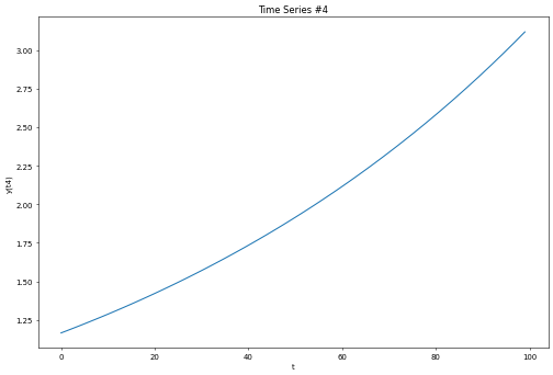
Exponential Growth

As you might have previously noticed in the double exponential smoothing equation, the growth is modelled by noting the difference between the last smoothing statistic and the current smoothing statistic. This type of trend model will not suffice in cases where the growth rate is exponential.

Time Series #4 — Exponential Growth

In most modelling software packages one can therefore set the trend term to ‘multiplicative’. This allows the trend to be modelled based on percentage growth rates. Using a multiplicative trend term, we get the following forecast:

Much more reasonable.

Choosing Alpha, Beta & Gamma with AutoETS

Lastly, I have so far failed to mention how one can pick the best parameters alpha, beta and gamma for the models. Typically, these parameters can be found by back fitting the model to historical data and optimising for various metrics e.g. minimizing least squares, AIC, maximising the likelihood etc. Thankfully, there are many software packages available to do this quickly and easily.

If you are a Python user, the sktime package has an AutoETS function:

Welcome to sktime - sktime documentation

If you prefer R, the ‘forecast’ library has features to automatically estimate parameters:

forecast: Forecasting Functions for Time Series and Linear Models

More Information

The information in this post is a summary of the recent ‘Berlin Time Series Meetup’ session ‘Introduction to Forecasting’. If you are interested in Time Series and its applications, you can join us by clicking on the following link.

Berlin Time Series Analysis Meetup (Berlin, Germany)

In addition, code and example notebooks for this article can be found on our Github page:

btsa/python/intro_forecasting at master · juanitorduz/btsa

BTSA is a group of 4 Data Scientists in Berlin, interested in all things Time Series and related ML applications. If you wish to contact us for more information or questions, please reach out to us at

BTSA Contact: berlin.timeseries.analysis@gmail.com

Author:
Aaron Pickering
Co-founder @ Seenly

Further Reading

Recommended further reading:

‘Forecasting: Principles and Practice’ by Hyndman and Athanasopoulos is an excellent text and highly recommended.

Forecasting: Principles and Practice (3rd ed)

Hyndman, R.J., & Athanasopoulos, G. (2021) Forecasting: principles and practice, 3rd edition, OTexts: Melbourne, Australia. OTexts.com/fpp3

‘Introduction to Time Series and Forecasting’ by Davis and Brockwell.

Introduction to Time Series and Forecasting